As part of Fathom’s presence at #EGU22 in Vienna, Chief Research Officer Dr Oliver Wing presents our collaboration with Deltares and AXA to develop a European catastrophe model.
This presentation is part of Fathom’s presence at #EGU22 in Vienna, Austria.
Video transcript
0:01 Hello everyone. My name’s Ollie Wing and I’m the Chief Research Officer at Fathom. In this presentation I’ll be discussing a really exciting collaboration between fathom a flood risk modelling company in Bristol that I work for…
0:13 Deltares, a flood modeling firm in the Netherlands, and AXA’s catastrophe flood modelling team based in Paris. I’m merely the messenger of this excellent bit of science leaning on the expertise of all of those listed here. So thanks to Hessell, Hélène, Mark, and Albrecht at Deltares, Rémi, Hugo and Anna at AXA and Andy and Chris at Fathom.
0:36 So just start with, I’ll give you the grand overview of the approach to build a European flood catastrophe model. A catastrophe model differs from other hazard or risk models by simulating long synthetic sets of plausible flood events.
0:49 Without understanding spatial correlation, you kind of understand the extreme losses at the top then is a stochastic weather generator developed by AXA.
0:58 This produces plausible weather patterns using a temporal reshuffling of historical data. Deltares’ hydrological model consumes these 10,000 years of weather patterns and turns those into 10,000 years of stream flow.
1:12 All the while Fathom are producing return period flood maps to yield a catalog of flood intensity probabilities. The 10,000 year time series is then used to sample from a hazard maps in space per event.
1:26 So onto the weather generator, we developed a time re-sampling stochastic weather generator based on weather regimes and wet, dry alternation.
1:35 It takes into account precipitation, persistence and preserves, historical observed statistics and extremes across Europe. 10,000 years of synthetic weather is therefore reproduced. This model, essentially temporarily reshuffles era five re-analysis data entire days of weather, are sampled from continent wide and re concatenate it to produce new multi-day extremes.
1:59 The reshuffling is based on three parameters, the clustering of historical data into weather regimes based on multiple variables that trigger precipitation at the European scale.
2:09 Second clustering based only on precipitation patterns at a finer geographic scale and dry and wet sequences of precipitation based on historical distribution.
2:21 With this approach, we can generate new sequences of precipitation accumulation. You can see here, for instance, the 200 year precipitation accumulation across 10 days, this plot using the Rhine basin as an example, shows how historical precipitation accumulations across 10 days, the red crosses are extended to produce new and unseen 10 day extremes.
2:44 Meanwhile, the spacial coherence at the flood events is implicitly retained. Deltares’ distributed hydrological model wflow then simulates the river flow response to these synthetic weather patterns.
2:57 It does this at two kilometer resolution so that the information content at high resolutions is also preserved as a neat upscaling algorithm applied. Before the 10,000 year run though, as with all hydrological models…
3:10 …it needs to be calibrated for this Deltares used pedo-transfer functions. Given the spatial scale of this model, we are not seeking a very heavy calibration to river gauges, but rather the approach was more like a sensitivity analysis to select sensible basin-wide pedo-transfer parameters to maintain continent wide spacial coherence. As such, the approach slip to the parameter, which describes the relationship between horizontal and vertical conductivity of water in the subsurface, optimal parameters where each basin where linked to existing constraint parameters to produce a coherent continental parameter set. Some of the Kling-Gupta efficiency scores for river gauges in particular countries are shown here, the key plot, give a great example of the philosophy of this modelling approach.
4:01 You can see that for this particular station in those first two plots that there’s an obvious model bias, wflows over predicting flood response. But that right base plot shows the return period calculated internally to model an observation separately of each flood event.
4:18 You can see here that while those absolute discharges are biased, the relative frequencies of their exceedance are not. The reason why this is important will come in a second.
4:28 Next up, we have Fathom’s principle contribution to the project, the hydraulic modelling. We’re producing multiple return period, flood depth grids across the continent at one up second resolution.
4:40 River flows are estimated using the Zhao et al., 2021 regional flood frequency analysis, and pluvial intensity duration, frequency relationships, are estimated in a similar vein using a machine learning approach to regionalize IDF curves computed from sub daily rain gauges. Terrain data is drawn from LIDAR, where we can find it using FABDEM, which is the Copernicus DSM, (which some of you might also know as tandem X) with forest and buildings removed as the data set of last resort.
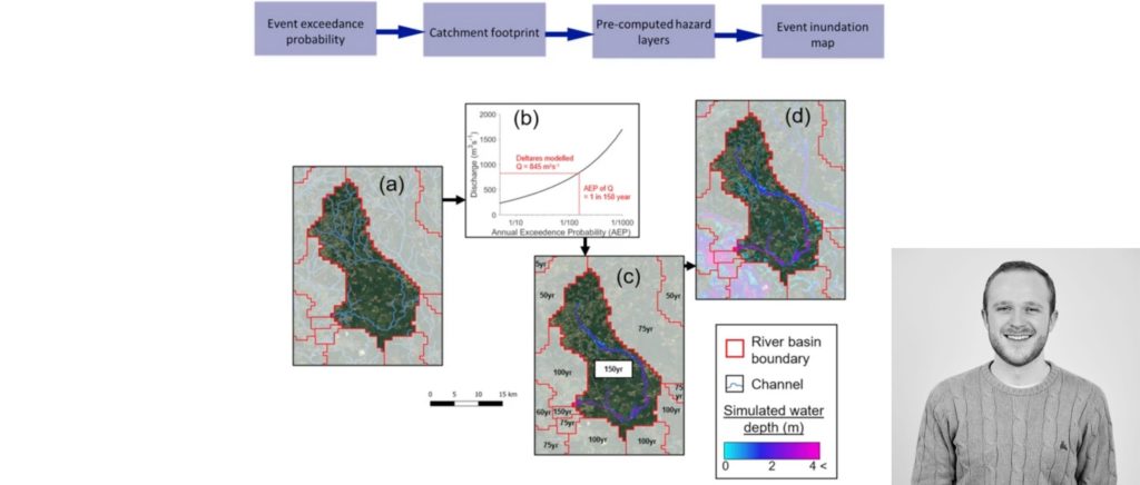
5:12 The way we construct for events is adopting the so-called cookie cutter approach. This involves segmenting the hazard data from previously into sub catchments.
5:22 And when an event described by its relative frequency or return period in the 10,000 year hundred metric time series occurs, we cut out the relevant flood map within that catchment and paste it into the event footprint.
5:35 We repeat that for all impacted catchments and all events. Since we are matching return periods on this stochastic model to return periods in the hydraulic model, that’s why spacial coherence and relative frequencies are so important.
5:50 We’ve done some validation of these flood maps. This uses the calibrated historical hindcast simulated by debris flow. And from that extract events, for which we have referenced data to benchmark the model. You can see here, for instance, the discharge simulation for a flood in Germany, we identify the return period of that event in that catchment.
6:09 And then repeat to reconstruct the flood event. This graph is also a good illustration of the need for a 10,000 years stochastic model.
6:18 You can see this event was unprecedented around an 8,000 year return period, but the parameter estimates are really unstable based on only a few decades of flow data with 10,000 years of flows, we can instead empirically understand the frequency of that event. Anyway, onto the validation.
6:35 There are 10 events that we tested against within which there are lots of sub-domains in different types of data to test with.
6:48 For events, which we had a water level observations for on average, across all events, we got around a metre of model errors. While that seems a lot, it’s worth bearing in mind, the considerable error in the benchmarks themselves, separate studies show high watermark based water level measurements can be subject to half to one meter of error.
7:08 Similarly, we evaluated further steps and less discriminatory tested the model, but it does tell us if we broadening matching the local spatial patterns of historical floods, note that errors in flood extent, imagery as such that two independent classifications or images at the same flood often have around 75% similarity.
7:27 We find on average flood extent similarity accounting for both under and over prediction of errors of around two thirds. Ignoring over prediction, which can be unreliably tested by these benchmark datasets, 85% of wet pixels are captured by the models.
7:44 These numbers are about in line with the expectations for a model of this scope and scale.
7:51 And that’s it. There’s still a lot of work left to do in this project. All these components need bringing together along with vulnerability functions to generate the catastrophe model.
8:01 Plus we have the small issue of creating climate conditioned events sets, where we can explore the impact of projected climate change on European flood.
8:09 If you have any questions, please do just talk to me or drop me an email. Thank you.